Introduction

Diffusion (Sohl-Dickstein et al. 2015; Song and Ermon 2020; Ho, Jain, and Abbeel 2020) and Flow Matching (Liu, Gong, and Liu 2022; Albergo and Vanden-Eijnden 2023; Lipman et al. 2023) provide a stable and general approach for learning models of continuous data distributions. However, their efficiency is highly dependent on the data representation. Latent Diffusion Models (LDMs) (Rombach et al. 2022) reduce computational demands significantly by working in a latent space where images can be encoded to and decoded from. The latent space is learned with a variational autoencoder (VAE) (Diederik P. Kingma and Welling 2022; Rezende, Mohamed, and Wierstra 2014) using a combination of pixel-wise regression, perceptual feature losses (Johnson, Alahi, and Fei-Fei 2016) and an adversarial objective (Goodfellow et al. 2014; Esser, Rombach, and Ommer 2021). This enables high-fidelity reconstructions from a latent representation that focuses on perceptually relevant features while discarding imperceptible noise in the original signal (Dieleman 2025).

While such “perceptual representations” significantly reduce the computational requirements, recent works demonstrated how “semantic representations” (Zheng et al. 2025; Leng et al. 2025) can result in yet another major efficiency boost.

The Learnability-Quality-Compression Trade-off

When designing latent representations for generative models, we face a fundamental three-way trade-off between:

Learnability (Semantic Spaces): How easily can a generative model learn to produce new samples in the latent space? Semantic representations may simplify the modeling task, as the generative model only needs to capture high-level semantic relationships rather than low-level perceptual details (Dieleman 2025), but may reduce both quality and compression rate.
Quality (Perceptual Distortion): How faithfully can the decoder reconstruct the original signal from its latent representation? Aggressive compression often leads to perceptual distortions and loss of fine-grained details. Autoencoders trained with perceptual and adversarial losses help maintain reconstruction quality, but increasing compression inevitably degrades fidelity. Furthermore, autoencoders that prioritize reconstruction fidelity without explicit regularization toward semantically meaningful representations may produce latent spaces with high-frequency or irregular structures that are challenging for generative models to learn.
Compression (Rate): How much can we reduce the dimensionality of the latent space? Higher compression rates can improve modeling effciency, but may hurt both reconstruction quality and the generative model’s ability to capture the full distribution (Zheng et al. 2025).

These three objectives are inherently conflicting: increasing compression (rate) typically degrades reconstruction quality and may harm learnability; optimizing for perfect reconstructions requires less compression; and maximizing learnability through semantic structure may require sacrificing low-level perceptual fidelity. This suggests that the optimal trade-off lies in discarding imperceptible information while preserving semantically meaningful structure that generative models can efficiently learn.

In this blog post, we provide an in-depth analysis of this three-way trade-off. We train flow matching models in the latent space of various autoencoders with different capacity and design choices. Figure 1 shows that the FLUX.2 AE provides the most balanced approach, resulting in highest quality generations and relatively modest training times. These findings provide grounds for future work, which we briefly discuss in the end of this blog.

Code

import pandas as pd
from itables import show
import plotly.graph_objects as go


df = pd.read_parquet("../data")

best = df.copy()
best = best.loc[best.groupby(["step", "ae", "repa"]).fid.idxmin()]

fig = go.Figure()

data = [
    ("FLUX.2", 3.701722, 0.2668),
    ("FLUX.1", 10.12791, 0.3380),
    ("SD", 7.72709, 0.9519),
    ("RAE", 3.103955, 1.6737),
]

flux2_gfid, flux2_pdist = data[0][1], data[0][2]

for ae, gfid, pdist in data:
    fig.add_trace(
        go.Scatter(
            x=[gfid],
            y=[pdist],
            mode="markers+text",
            name=ae,
            text=[ae],
            textposition="top center",
            showlegend=False,
            marker=dict(size=12),
            hovertemplate='gFID: %{x}<br>LPIPS: %{y} <extra></extra>',
        )
    )

    if ae != "FLUX.2":
        fig.add_trace(
            go.Scatter(
                x=[flux2_gfid, gfid],
                y=[flux2_pdist, pdist],
                mode="lines",
                showlegend=False,
                line=dict(color="gray", width=1),
                hoverinfo="skip",
            )
        )

        mid_x = (flux2_gfid + gfid) / 2
        mid_y = (flux2_pdist + pdist) / 2
        gfid_change = ((flux2_gfid - gfid) / gfid) * 100
        pdist_change = ((flux2_pdist - pdist) / pdist) * 100

        gfid_color = "green" if gfid_change < 0 else "red"
        pdist_color = "green" if pdist_change < 0 else "red"

        fig.add_annotation(
            x=mid_x,
            y=mid_y,
            text=f"{ae} → FLUX.2<br>gFID: <span style='color:{gfid_color}'>{gfid_change:+.1f}%</span><br>LPIPS: <span style='color:{pdist_color}'>{pdist_change:+.1f}%</span>",
            showarrow=False,
            bgcolor="white",
            bordercolor="gray",
            borderwidth=1,
        )

fig.update_layout(
    xaxis_title="Learnability (gFID ↓)",
    yaxis_title="Fidelity (LPIPS ↓)",
    title="Learnability vs Fidelity",
    hoverlabel=dict(namelength=-1),
    showlegend=False,
)
fig.show()

Figure 1: Results from our analysis of the trade-off between reconstruction fidelity (as measured by LPIPS) and learnability (as measured by generative FID, gFID). While FLUX.1 obtains significant improvements in reconstruction fidelity over the SD AE, it achieves this at the cost of worse learnability. On the other extreme, RAE demonstrates excellent learnability properties but has to trade this improvement for degraded reconstruction capabilities. In contrast, FLUX.2 shows improved learnability over FLUX.1 and SD while simultaneously improving reconstruction capabilities over all of the three other AEs.

Experiments

To evaluate the “learnability” (Yao, Yang, and Wang 2025; Kouzelis, Kakogeorgiou, et al. 2025; Skorokhodov et al. 2025; Zhou et al. 2025; Leng et al. 2025; Zheng et al. 2025) of different representations, we follow a latent flow matching (Esser et al. 2024; Ma et al. 2024; Lipman et al. 2023; Liu, Gong, and Liu 2022) setup. To isolate the effect of the representations, most hyperparameters and architecture choices are kept constant. Following DiT/SiT (Peebles and Xie 2023; Ma et al. 2024), we train on ImageNet and use a constant learning rate of \(10^{−4}\), no weight decay, a batch size of 256 and an EMA decay of \(0.9999\). We optimize the parameters \(\theta\) of a DiT-XL backbone \(v_\theta\) architecture over the conditional flow matching (CFM) loss:

\[ \mathcal{L}_\text{CFM}(\theta) = \mathbb{E}_{t\sim p,u \sim p_\text{data},\epsilon \sim \mathcal{N}} \Vert v_\theta((1 - t) E(u) + t \epsilon; t) - (\epsilon - E(u)) \Vert^2, \]

where \(E\) is a frozen image encoder (as described in Autoencoders), \(\mathcal{N}\) is a standard normal distribution for sampling noise, \(p_\text{data}\) is the Imagenet training data at resolution \(256 \times 256\). \(p\) is the distribution used for sampling timesteps \(t\) during training. As \(t\) determines the signal-noise-ratio of the input, \(v_t = (1 - t) E(u) + t \epsilon\), the choice of \(p\) can significantly affect the training dynamics and final performance (Diederik P. Kingma and Gao 2023; Zeng and Yan 2025). Moreover, its optimal choice depends on data properties such as resolution (Hoogeboom, Heek, and Salimans 2023) but also on properties of the data representation such as its scale (Karras et al. 2022), dimensionality (Zheng et al. 2025) and spectrum (Falck et al. 2025). Thus, to enable a fair comparison across different representations, we train each representation with multiple choices for \(p\) to enable a comparison under (approximately) optimal choices.

For evaluations, we sample models every 100k steps using a fixed inference budget of 50 Euler steps. We compute FID (Heusel et al. 2018) between 50k samples produced with randomly sampled ImageNet classes (as opposed to class-balanced sampling as in (Zheng et al. 2025)) and the reference batch provided by ADM (Dhariwal and Nichol 2021). Similar to the training distribution for timesteps, the optimal sampling grid also depends on the representation and we search over various sampling timestep variants.

Next, we describe the choices of training and sampling timesteps that we consider in our study.

Sampling Shifts

The timeshift function is

\[ s(\alpha, \cdot): t \mapsto \frac{\alpha t}{1 + (\alpha - 1) t} \]

Consider a random variable \(Y(t) = (1-t)c + t\eta\), where \(c \in \mathbb{R}, \eta \sim \mathcal{N}(0, 1)\). Then, the error between \(c\) and its sample estimate from \(n\) observations \((y_{t,i})_{i=1}^{n}\) of \(Y(t)\), \(\hat{c}(n) = \frac{1}{1-t} \frac{1}{n} \sum_{i=1}^{n} y_{t,i}\), has a standard deviation of \(\sigma(t, n) = \frac{t}{1-t}\sqrt{\frac{1}{n}}\). Thus

\[ \sigma(t, n) = \sigma(s({\sqrt{\frac{m}{n}}}, t), m), \]

i.e. \(s\) provides the timeshift necessary to keep the uncertainty identical between \(n\) and \(m\) observations (Esser et al. 2024), which can serve as a simple model for the shift required under different resolutions (Hoogeboom, Heek, and Salimans 2023) and which has also been shown empirically to predict the shift required for higher dimensional representations (Yu et al. 2025).

Note

The form of the sample estimate \(\hat{c}\) follows from the relationship \(\mathbb{E} Y(t) = (1-t)c\) and its standard deviation then from \(\text{Var}(Y(t)) = t^2\) and the standard error from the mean.

We consider \(\alpha \in \{1.00, 1.78, 2.95, 4.63, 6.93\}\), which gives the following shapes for \(s\):

Code

import numpy as np
import plotly.graph_objects as go


def timeshift(alpha, t):
    return alpha * t / (1.0 + (alpha - 1.0) * t)


alphas = [1.00, 1.78, 2.95, 4.63, 6.93]
ts = np.linspace(0, 1, 100)

fig = go.Figure()
for alpha in alphas:
    fig.add_trace(
        go.Scatter(
            x=ts,
            y=timeshift(alpha, ts),
            mode="lines",
            name=f"s({alpha}, ·)",
            opacity=1,
        )
    )
    fig.update_layout(
        xaxis_title="t",
        yaxis_title="s",
        title="Timeshift function",
        hoverlabel=dict(namelength=-1),
        showlegend=True,
    )
fig.show()

Training Distributions

We consider different ways to sample noise timesteps for training.

Shifted Uniform

Here, we combine a uniform timestep sampling with the shifting function \(s\), which gives

\[ \begin{gather} t = s(\alpha, u), u \sim \mathcal{U}(0, 1) \\ \iff \\ t \sim p_\text{ts}(t; \alpha) = \frac{\alpha}{(\alpha + (1-\alpha)t)^2} \end{gather} \]

Note

Follows directly from the change of variables for probability density functions,

\[ y = f(x), x \sim p_X(x) \implies y \sim p_Y(y) = p_X(f^{-1}(y)) \left| (f^{-1})'(y) \right| \]

and the inverse of \(s\):

\[ s(\alpha, \cdot)^{-1}(u) = \frac{\frac{1}{\alpha}u}{1+(\frac{1}{\alpha} - 1)u} = s(\frac{1}{\alpha}, u) \]

which looks like this for our values of \(\alpha\):

Code

def shifted_uniform(alpha, t):
    return alpha / (alpha + (1.0 - alpha) * t)**2


alphas = [1.00, 1.78, 2.95, 4.63, 6.93]
ts = np.linspace(0, 1, 100)

fig = go.Figure()
for alpha in alphas:
    fig.add_trace(
        go.Scatter(
            x=ts,
            y=shifted_uniform(alpha, ts),
            mode="lines",
            name=f"p_ts(·, {alpha})",
            opacity=1,
        )
    )
    fig.update_layout(
        xaxis_title="t",
        yaxis_title="p_ts",
        title="Shifted uniform density",
        hoverlabel=dict(namelength=-1),
        showlegend=True,
    )
fig.show()

Note that this is the distribution proposed for training in (Zheng et al. 2025).

Shifted Logit Normal

When considering the logit-normal distribution,

\[ p_\text{ln}(t; \mu, \sigma) = \frac{1}{\sigma \sqrt{2\pi}} \frac{1}{t(1-t)}\exp\left(-\frac{(\text{logit}(t) - \mu)^2}{2s^2}\right) \]

with \(\text{logit}(t) = \log\frac{t}{1-t}\), sampling from this distribution followed by a timeshift is equivalent to sampling from the logit-normal distribution with \(\mu\) shifted by \(\log\alpha\) (Labs et al. 2025):

\[ \begin{gather} t = s(\alpha, u), u \sim p_\text{ln}(u; \mu, \sigma) \\ \iff \\ t \sim p_\text{ln}(t; \mu + \log\alpha, \sigma) \end{gather} \]

This gives the following densities for our experiments:

Code

def logit_normal(t, mu, sigma):
    return np.exp(-(np.log(t/(1-t)) - mu)**2/(2*sigma**2))/(t * (1 - t))/(sigma*np.sqrt(2*np.pi))


alphas = [1.00, 1.78, 2.95, 4.63, 6.93]
ts = np.linspace(0, 1, 100)

fig = go.Figure()
for alpha in alphas:
    fig.add_trace(
        go.Scatter(
            x=ts,
            y=logit_normal(ts, mu=np.log(alpha), sigma=1.0),
            mode="lines",
            name=f"p_ln(·, {alpha})",
            opacity=1,
        )
    )
    fig.update_layout(
        xaxis_title="t",
        yaxis_title="p_ln",
        title="Shifted logit normal density",
        hoverlabel=dict(namelength=-1),
        showlegend=True,
    )
fig.show()

Plateau Logit Normal

Here, we consider a variant of the logit-normal sampler that biases sampling towards high noise timesteps by remaining constant after its mode:

Code

import math
from functools import lru_cache
from scipy import integrate


def ln_cdf(t, mu, sigma):
    result, _ = integrate.quad(lambda x: logit_normal(x, mu, sigma), 0.0, t)
    return result


@lru_cache(maxsize=None)
def tpPln(mu, sigma):
    # mode
    t_star = 1 / (1 + np.exp(-mu))
    for _ in range(20):
        g = np.log(t_star / (1 - t_star)) - mu - (2 * t_star - 1)
        dg = 1 / (t_star * (1 - t_star)) - 2
        t_star = np.clip(t_star - g / dg, a_min=1e-6, a_max=1 - 1e-6)

    p_ln = logit_normal(t_star, mu, sigma)
    P_ln = ln_cdf(t_star, mu, sigma)
    return t_star, p_ln, P_ln


def plateau_logit_normal(t, mu, sigma):
    t_star, p_ln, P_ln = tpPln(mu, sigma)
    Z = P_ln + (1 - t_star) * p_ln

    t = np.clip(t, a_min=1e-6, a_max=t_star - 1e-6)

    return logit_normal(t, mu, sigma) / Z


alphas = [1.00, 1.78, 2.95, 4.63, 6.93]
ts = np.linspace(0, 1, 100)

fig = go.Figure()
for alpha in alphas:
    fig.add_trace(
        go.Scatter(
            x=ts,
            y=plateau_logit_normal(ts, mu=np.log(alpha), sigma=1.0),
            mode="lines",
            name=f"p_ln(·, {alpha})",
            opacity=1,
        )
    )
    fig.update_layout(
        xaxis_title="t",
        yaxis_title="p_ln",
        title="Shifted logit normal density",
        hoverlabel=dict(namelength=-1),
        showlegend=True,
    )
fig.show()

Autoencoders

Latent generative models (Dai and Wipf 2019) utilize autoencoders (AEs), consisting of an encoder \(E\) mapping the original data \(u\) to a latent representation \(E(u)\) and a decoder \(D\) approximately inverting \(E\) to obtain reconstructions \(\tilde{u} \simeq D(E(u))\). The goal is to model the data distribution in a latent space with better properties compared to the original data representation.

A common approach is to train \(E\) and \(D\) jointly for the reconstruction task. A reduction of the latent dimensionality, i.e. \(\text{dim} E(u) < \text{dim} u\), and a distributional regularization, using a Kullback-Leibler divergence, introduce an Information Bottleneck that regularizes the latent space. In combination with perceptual feature losses and adversarial training for the reconstruction task, this leads to a perceptually compressed representation that improves the efficiency of generative modeling by focusing on perceptually relevant features of the data.

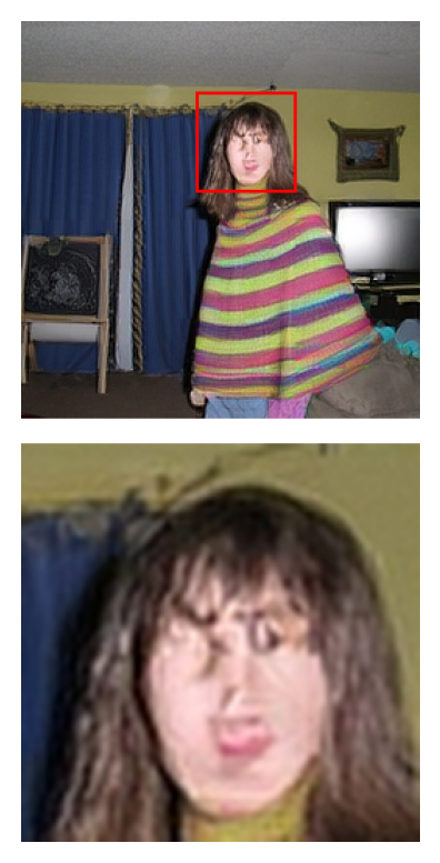
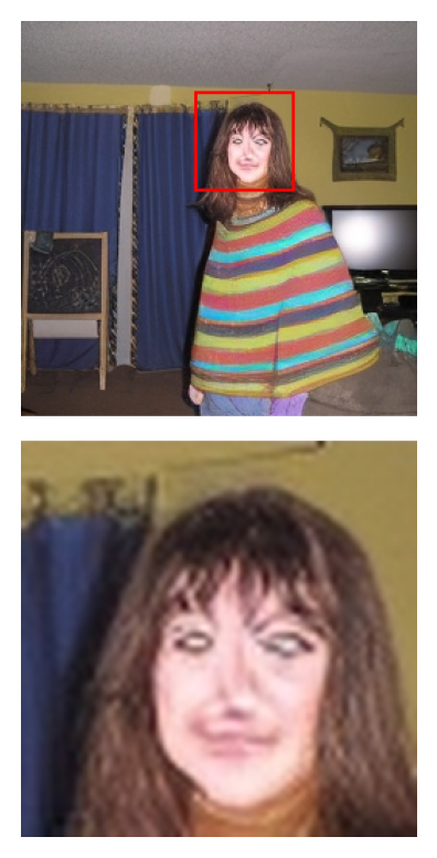
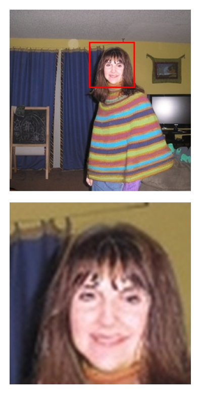
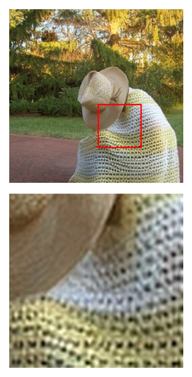
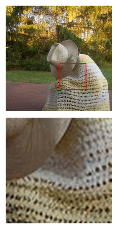
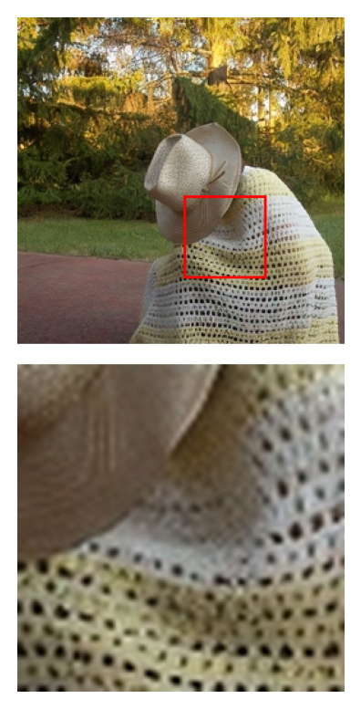
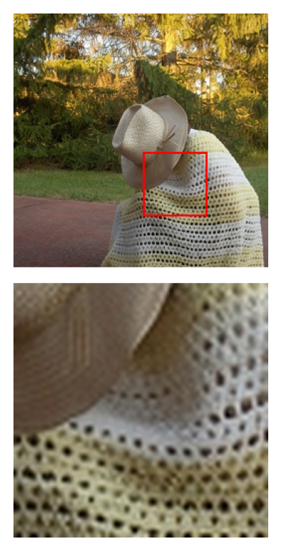
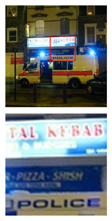
We include two variants of this approach, the SD-VAE and the FLUX.1-VAE from FLUX.1 (Labs 2024) and FLUX.1 Kontext (Labs et al. 2025). Both AEs closely follow the design and training of (Rombach et al. 2022). Since image-editing applications in FLUX.1 Kontext require high-fidelity reconstructions of inputs, the FLUX.1 VAE had to widen the Information Bottleneck to shift the trade-off between compression and quality towards the latter. Consequently, the FLUX.1 VAE was trained with a 4x larger latent dimensionality and reduced regularization weight. The reconstruction metrics in Table 1 show that this design choice indeed reduces perceptual distortion and thus opens the possibility of high-fidelity image editing. However, since the now weakened Information Bottleneck is the only means of improving the quality of the latent space in this approach, the results in Figure 1 and Figure 2 demonstrate that these same choices also result in reduced learnability of the latent space.

Different lines of works go beyond this relatively simple Information Bottleneck and consider other properties and approaches that affect the learnability of representations. One line of work starts from a spectral analysis of representations (Dieleman 2024; Gerdes, Welling, and Cheng 2024). Besides direct intervention in spectral properties (Falck et al. 2025), these considerations often lead to regularizations aiming to make representations more equivariant with image transformations (Skorokhodov et al. 2025; Zhou et al. 2025; Kouzelis, Kakogeorgiou, et al. 2025). Another line of work focuses on semantic qualities of representations. Starting with the insights from (Yu et al. 2025), that alignment of diffusion model features with vision foundation (VF) models such as DINOv2 (Oquab et al. 2023) leads to significant performance improvements, (Yao, Yang, and Wang 2025) applies such an alignment directly to the VAE training, resulting in a significantly more effective regularization compared to the Information Bottleneck from above. Similarly, other works combine autoencoder representations with more semantic modalities (Chefer et al. 2025) or VF features Wu et al. (2025). (Leng et al. 2025) demonstrates that the REPA objective of (Yu et al. 2025) enables end-to-end training of VAEs with latent diffusion models, which provides a more direct way to optimize for learnability. We integrate these insights into the FLUX.2 VAE to develop a representation that satisifes the high-fidelity requirements imposed by image-editing, while simultaneously improving learnability properties. By reducing the compression with a 8x larger dimensionality compared to the SD-VAE, Table 1 shows that FLUX.2 improves reconstruction fidelity further beyond the FLUX.1 VAE, while Figure 1 and Figure 2 show that the introduction of semantic regularization leads to improved learnability.

Recent works present approaches where a VF representation is used directly. (Zheng et al. 2025) uses a frozen VF encoder as the encoder and then learn a decoder for it to obtain a Representation Autoencoder (RAE). RepTok (Gui et al. 2025) adapts a single token from a VF into an autoencoder representation enabling highly efficient training of generative models. However, while these approaches lead to impressive learnability properties (as shown in Figure 1 and Figure 2 for RAE), the extreme compression of RepTok and the complete absence of a pixel reconstruction objective for RAE’s encoder lead to decreased reconstruction fidelity as shown in Table 1. We include RAE as a representative variant in our study, as RepTok reports an even lower rFID of 1.85 compared to RAE’s 0.57.

Note that we follow (Peebles and Xie 2023) and use a \(2 \times 2\) patching for the latent representations of SD, FLUX.1 and FLUX.2 AE. As in (Zheng et al. 2025), we use no patching for RAE, as this leads to a consistent sequence length of 256 tokens across all the considered AEs. In this configuration, SD produces 16, FLUX.1 64, FLUX.2 128, and RAE 768 channels per token.

Reconstruction Performance

We evaluate reconstruction fidelity with the reference-based metrics LPIPS (Zhang et al. 2018), Structural Similarity (SSIM) (Wang et al. 2004) and Peak Signal-to-Noise Ratio (PSNR). For non-reference based evaluation, we compute the reconstruction FID (rFID). All metrics are computed on the ImageNet validation set. The results in Table 1 demonstrate how FLUX.1 and FLUX.2 AEs improve all metrics over the SD AE, whereas for RAE, we observe an improvement in the non-reference based metric rFID despite worse performance in reference based metrics. While good rFID scores can indicate suitability for general modeling tasks, some applications such as image editing rely on high-fidelity reconstructions as measured by reference based metrics.

Table 1: Reconstruction metrics of the different autoencoders on the ImageNet validation set. We include the original rFID reported by (Yu et al. 2025) for RAE and SD in parentheses.

Model	LPIPS	SSIM	PSNR	rFID
RAE	1.6737 ± 0.0057	0.4962 ± 0.0026	18.8272 ± 0.0429	0.6107 (0.57)
SD	0.9519 ± 0.0054	0.6976 ± 0.0121	25.0520 ± 0.0673	0.6451 (0.62)
FLUX.1	0.3380 ± 0.0026	0.8893 ± 0.0058	31.1312 ± 0.0745	0.1761
FLUX.2	0.2668 ± 0.0017	0.9038 ± 0.0049	31.4632 ± 0.0633	0.1124

Qualitative

Code

from PIL import Image, ImageDraw
import plotly.express as px
import matplotlib.pyplot as plt

def imshow(img):
    plt.figure()
    plt.imshow(img, aspect="equal")
    plt.axis("off")
    plt.show()

def draw_box_with_zoom(img, padding, box):
    left, top, size = box

    output_height = 2 * img.height + padding
    output = Image.new('RGB', (img.width, output_height), 'white')

    output.paste(img, (0, 0))

    draw = ImageDraw.Draw(output)
    draw.rectangle([left, top, left + size, top + size], outline='red', width=2)

    box_region = img.crop((left, top, left + size, top + size))
    zoomed = box_region.resize((img.width, img.height), Image.LANCZOS)

    output.paste(zoomed, (0, img.height + padding))

    return output

boxes = [
    (112, 46, 64),
    (130, 140, 64),
    (112, 76, 64),
]
for i, box in enumerate(boxes):
    for name in ["orig", "rae", "sd", "flux1", "flux2"]:
        img = Image.open(f"../imgs/{name}-{i:02}.png")
        imshow(draw_box_with_zoom(img, 16, box))

Results

We plot the FID evaluation results as they progress over time in Figure 2. For each representation, we have 30 different runs consisting of 3 different training distributions, 5 different training shifts, 5 different sampling shifts and one variant with a REPA alignment objective (Yu et al. 2025) and one without.

We observe that evaluating the quality of representations for generation faithfully requires a tuning over timestep distributions. Furthermore, we see that REPA consistently improves the performance for all representations. This even holds for RAE, where both the logit-normal timestep sampling and the additional REPA objective improve performance over the settings proposed in (Zheng et al. 2025). While featuring significantly improved reconstruction performance, the FLUX.2 AE reaches learnability levels close to those of RAE with the original settings.

Code

colors = {
  ("flux2", "none"): "blue",
  ("flux2", "dinov2b"): "cyan",
  ("flux1", "none"): "orange",
  ("flux1", "dinov2b"): "magenta",
  ("rae", "none"): "red",
  ("rae", "dinov2b"): "purple",
  ("sd", "none"): "green",
  ("sd", "dinov2b"): "brown",
}


fig = go.Figure()

# all in background
for name, group in df.groupby(["ae", "repa", "trainp", "trainshift", "sampleshift"]):
    colorname = (name[0], name[1])
    fig.add_trace(
        go.Scatter(
            x=group["step"],
            y=group["fid"],
            mode="lines",
            opacity=0.03,
            line=dict(color=colors[colorname]),
            showlegend=False,
            hoverinfo="skip",
        )
    )

# no shift
for name, group in df[(df["trainp"] == "ts") & (df["trainshift"] == 1.0) & (df["sampleshift"] == 1.0)].groupby(["ae", "repa", "trainp"]):
    colorname = (name[0], name[1])
    name = name[0] + ("" if name[1] == "none" else " + repa")
    fig.add_trace(
        go.Scatter(
            x=group["step"],
            y=group["fid"],
            mode="lines",
            opacity=0.5,
            line=dict(color=colors[colorname], dash="dot"),
            name=f"{name} (no shift)",
        )
    )

# rae in original setting
for name, group in df[(df["trainp"] == "ts") & (df["trainshift"] == 6.93) & (df["sampleshift"] == 6.93) & (df["ae"] == "rae")].groupby(["ae", "repa"]):
    colorname = (name[0], name[1])
    name = name[0] + ("" if name[1] == "none" else " + repa")
    fig.add_trace(
        go.Scatter(
            x=group["step"],
            y=group["fid"],
            mode="lines",
            opacity=0.5,
            line=dict(color=colors[colorname], dash="dashdot"),
            name=f"{name} (original shift)",
        )
    )

# best
for name, group in best.groupby(["ae", "repa"]):
    colorname = (name[0], name[1])
    name = name[0] + ("" if name[1] == "none" else " + repa")
    fig.add_trace(
        go.Scatter(
            x=group["step"],
            y=group["fid"],
            mode="lines",
            name=f"{name} (best shift)",
            opacity=1,
            line=dict(color=colors[colorname]),
        )
    )

fig.update_layout(
    xaxis_title="step",
    yaxis_title="FID",
    title="FID over training progress",
    hoverlabel=dict(namelength=-1),
    showlegend=True,
    yaxis=dict(range=[0.9 * best["fid"].min(), 0.66 * best["fid"].max()])
)
fig.show()

Figure 2: We train 4 different autoencoders with 15 different training timestep distributions (3 distributions, each with 5 shift parameters), with and without REPA (Yu et al. 2025), and evaluate them using 50 ODE sampling steps with 5 different sampling shift parameters. We highlight the performance under optimal settings (bold lines), the performance without any shifting (dotted lines) and, for RAE, the performance with the original parameters proposed in (Zheng et al. 2025) (dash-dotted lines). Depending on the parameter choice, the relative rankings can change. For example, without shifting, RAE perform worse than the FLUX.2 AE with shifting, whereas RAE outperforms the FLUX.2 AE if both are evaluated with optimal parameters.

Which parameters achieve the best performance?

In Table 2 we show the parameters that achieve the best performance for each step and autoencoder. We make four initial observations:

Only the logit-normal (ln) and the plateau-logit-normal (pln) distribution appear in the data. There always exists parameters for those that are better than a shifted uniform distribution.
While the choice between ln and pln distributions seems to change a bit, the training shift parameter remains constant except for one entry of the SD-AE, which prefers 1.78 at 200k steps, but otherwise 1.00. FLUX.2 AE performs best with 4.63 and RAE with 6.93. Thus, SD-AE and RAE are consistent with the \(\alpha=\sqrt{\frac{m}{n}}\) value that would be true under the simplified assumption of redundant data dimension, where \(n\) is the total dimensionality of the baseline (SD-AE with 16 channels) and \(m\) the increased dimension (768 for RAE). FLUX.2 prefers a slightly higher value than the predicted 2.82. However, if one considers reconstruction performance, it is plausible that FLUX.2 AE has a higher intrinsic dimensionality as it has significantly better reconstructions than SD-AE and RAE.
The choice of sampling shift parameter is similarly stable. Again, only the SD-VAE shows one exception, this time at step 100k, where it prefers 1.78 instead of 2.95. Both FLUX.2 and RAE perform best with 6.93. Thus, for sampling, all spaces prefer a slightly higher shifting compared to the train shift. It is likely that this is very dependent on the number of sampling steps and choice of sampler.
The shifting parameters remain mostly constant between runs with and without REPA, except for FLUX.1, where the optimal training shift reduces from 1.78 to 1.00 when adding the REPA objective. In combination with results from other AEs, where REPA does not change the optimal shifting parameters, one might conjecture that the REPA objective generally results in a small reduction of the optimal shifting value.

Code

table = best.copy()
table["name"] = table["ae"] + table["repa"].map(lambda x: " + repa" if x != "none" else "")
table = table[["name", "step", "trainp", "trainshift", "sampleshift", "fid"]]
table = table.sort_values(["name", "step"])
show(table, showIndex=False)

Table 2: For each autoencoder, we show the parameters that perform best with and without REPA across different steps.

Loading ITables v2.5.2 from the internet... (need help?)

How sensitive is performance to different parameters?

For practical guidance, we want to understand which parameters and choices matter most. We fix the step at 300k and, for each latent space (FLUX.1, FLUX.2, RAE and SD-VAE, in the columns), look at different parameters (training distribution, training shift and sampling shift, in the rows) in isolation.

For the training distribution, we observe a consistent gap between shifted uniform sampling (ts), and either logit-normal (ln) or plateau-logit-normal (pln) sampling. Among the latter two, logit-normal shows a bit better performance on FLUX.2 compared to pln, whereas for RAE, pln has minimally better performance. So to summarize, both ln and pln seem to work well and should be preferred over shifted uniform. When comparing best and worst training distribution, we see a 32.2% relative change for FLUX.2, 36.76% for FLUX.1, 6.8% for RAE and 19.8% for SD-VAE.

For the training shift, we see large performance differences if this parameter is not suitably chosen for the latent space. Qualitatively, the plots suggest the existence of an optimal value, and for RAE this might be even higher than the maximum considered value of 6.93. Performance between best and worst choices range from 61.5% (RAE) over 73.3% (FLUX.2), 75.7% (SD-VAE) to 86.42% (FLUX.1).

In line with the previous observations, the plots of the sampling shift parameter also suggest the existence of an optimal value which is likely to be a bit higher compared to the optimal training shift parameter. The relative differences are much lower here compared to the training shift parameter, with relatives changes from 4.5% (SD-VAE) over 6.8% (FLUX.1), 31.4% (FLUX.2) to 38.7% (RAE).

Code

subdf = df[df["step"] == 300000].copy()
subdf = subdf[subdf["ae"].isin(["flux2", "flux1", "rae", "sd"])]
subdf = subdf[subdf["repa"] == "none"]

# exclude outliers
subdf = subdf[(subdf["fid"] <= 50)]

for xcorrkey in ["trainp", "trainshift", "sampleshift"]:
    for ae in subdf["ae"].unique():
        fig = go.Figure()
        groupcols = [c for c in subdf.columns if c != xcorrkey and c != "ae" and c != "fid" and c != "repa"]
        for name, group in subdf[subdf["ae"] == ae].groupby(groupcols):
            legend = "|".join(map(lambda kv: f"{kv[0]}={kv[1]}", zip(groupcols, name)))
            group = group.sort_values([xcorrkey])
            fig.add_trace(
                go.Scatter(
                    x=group[xcorrkey],
                    y=group["fid"],
                    mode="markers",
                    name=legend,
                    opacity=1,
                )
            )
        fig.update_layout(
            xaxis_title=xcorrkey,
            yaxis_title="fid",
            title=f"Sensitivity of {xcorrkey} in {ae}",
            hoverlabel=dict(namelength=-1),
            showlegend=False,
        )
        if xcorrkey == "trainp":
            fig.update_xaxes(
                categoryorder="array",
                categoryarray= ["ts", "ln", "pln"],
            )
        fig.show()

Scaling Up: FLUX.2

Having established that the FLUX.2 autoencoder strikes a good balance in the learnability-quality trade-off, we now demonstrate how this representation enables state-of-the-art image generation and editing capabilities. Building on these foundations, we develop FLUX.2, a unified model family for both image generation and editing that combines our improved latent space with scale.

Architecture

FLUX.2 builds on a latent flow matching architecture (Lipman et al. 2023; Esser et al. 2024), and combines image generation and editing in a single unified model. The architecture couples the Mistral-3 24B parameter vision-language model (Mistral Small 3) with a rectified (Liu, Gong, and Liu 2022) flow transformer that incorporates modern activation functions (SwiGLU) and a more compute-efficient global modulation mechanism (Chen et al. 2025). The model operates in the FLUX.2 VAE latent space described earlier.

Evaluation

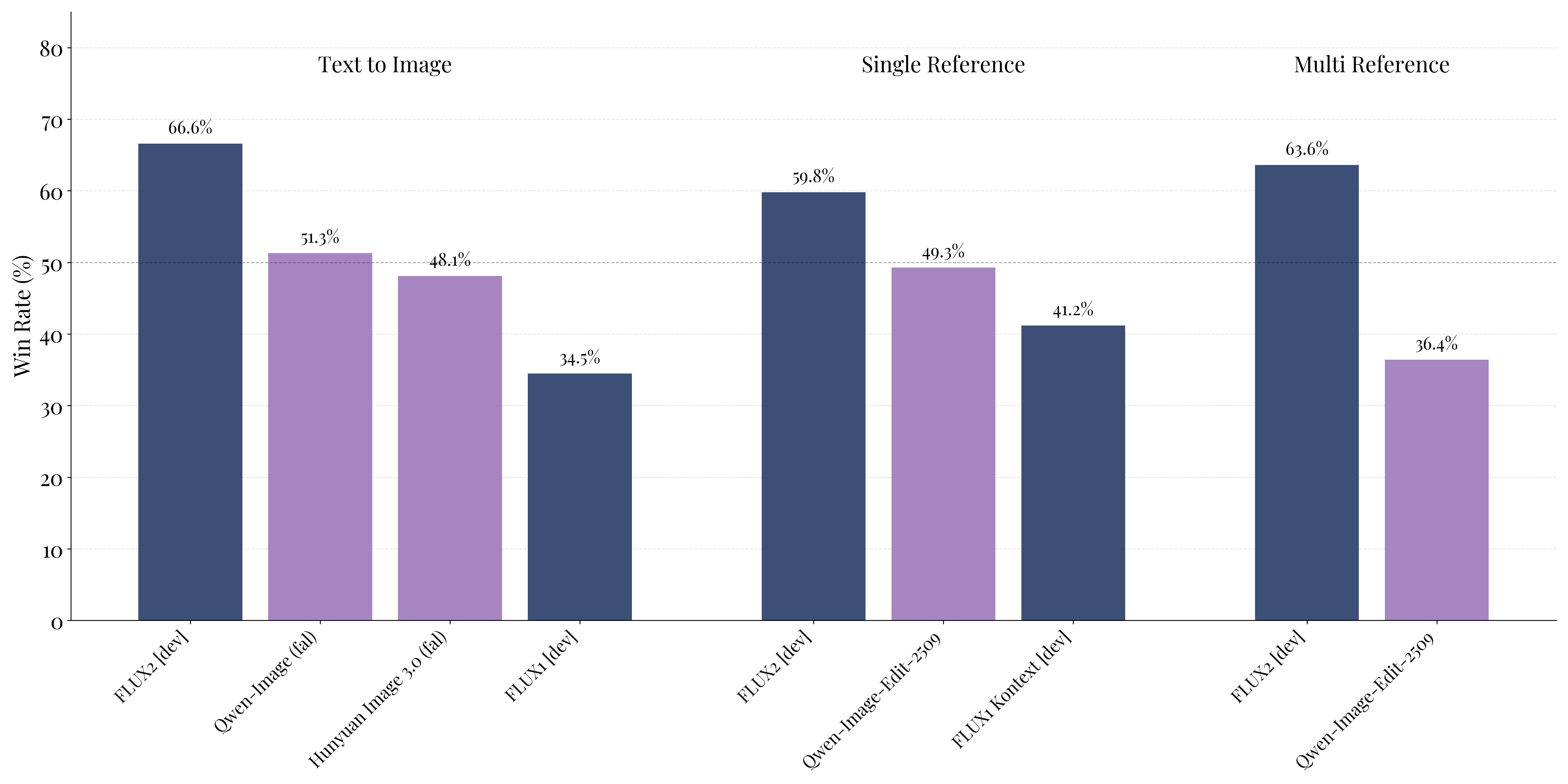
Figure 3 presents a comprehensive evaluation of FLUX.2 [dev] against leading open-source models across multiple benchmarks. The results demonstrate that FLUX.2 achieves state-of-the-art performance across diverse generation tasks, such as text-to-image generation and image editing with one or more refrerences.

More details about the FLUX.2 model family can be found in the official FLUX.2 announcement.

Limitations and Future Work

While the FLUX.2 VAE exhibits strong performance in both reconstruction quality and learnability, VAEs that sacrifice reconstruction quality continue to be more learnable. This motivates our continued efforts to further close the reconstruction-learnability gap without compromising either.

One promising direction for improving learnability is through enhanced diffusion representations. Recent work has demonstrated that enhancing representations can significantly boost diffusion model performance (Yu et al. 2025; Leng et al. 2025; Zheng et al. 2025). These approaches predominantly rely on external pretrained networks, achieving their best results with DINOv2 (Oquab et al. 2023) features, while focusing evaluations on ImageNet (Russakovsky et al. 2014). However, as we scale to larger, more diverse data distributions, it remains an open question whether approaches that do not enforce alignment with external feature networks such as DINOv2 can outperform those that do. Our preliminary scaling explorations for text-to-image generation suggest this might be the case: early results show superior generation quality for an alternative approach to REPA that does not rely on external representation learners. Figure 4 presents an initial comparison demonstrating improved performance without depending on pretrained feature extractors.

Stay tuned for FLUX.3 - coming soon ™.

Code

from IPython.display import HTML
from PIL import Image
import base64
from io import BytesIO

image_nums = [31, 36, 13, 44, 32, 40]

def img_to_base64(img_path):
    img = Image.open(img_path)
    buffered = BytesIO()
    img.save(buffered, format="JPEG")
    img_str = base64.b64encode(buffered.getvalue()).decode()
    return f"data:image/jpeg;base64,{img_str}"

html = """
<style>
.comparison-grid {
    display: grid;
    grid-template-columns: repeat(auto-fit, minmax(min(300px, 100%), 1fr));
    gap: 10px;
    width: 100%;
    align-items: center;
}
.comparison-pair {
    display: grid;
    grid-template-columns: 1fr 1fr;
    gap: 5px;
    align-items: center;
}
.comparison-pair > div {
    display: flex;
    flex-direction: column;
    align-items: center;
}
.comparison-pair img {
    width: 100%;
    height: auto;
    display: block;
}
.img-title {
    text-align: center;
    font-size: 11px;
    margin-bottom: 5px;
    font-weight: 500;
}
@media (max-width: 768px) {
    .comparison-grid {
        grid-template-columns: 1fr;
    }
}
</style>
<div class="comparison-grid">
"""

for i, img_num in enumerate(image_nums):
    repa_src = img_to_base64(f"../future_works_imgs/repa{img_num}.jpg")
    ours_src = img_to_base64(f"../future_works_imgs/ours{img_num}.jpg")

    html += f"""
    <div class="comparison-pair">
        <div>
            <div class="img-title">REPA (Yu et al. 2025)</div>
            <img src="{repa_src}" alt="REPA {img_num}">
        </div>
        <div>
            <div class="img-title">w/o external model</div>
            <img src="{ours_src}" alt="Ours {img_num}">
        </div>
    </div>
"""

html += "</div>"

display(HTML(html))

REPA 31 — Figure 4: Preliminary results comparing generation quality with and without REPA objective. Each pair shows REPA (left) vs our approach without external model (right) for the same prompt/seed.

Ours 31 — Figure 4: Preliminary results comparing generation quality with and without REPA objective. Each pair shows REPA (left) vs our approach without external model (right) for the same prompt/seed.

References

Albergo, Michael S., and Eric Vanden-Eijnden. 2023. “Building Normalizing Flows with Stochastic Interpolants.” https://arxiv.org/abs/2209.15571.

Chefer, Hila, Uriel Singer, Amit Zohar, Yuval Kirstain, Adam Polyak, Yaniv Taigman, Lior Wolf, and Shelly Sheynin. 2025. “VideoJAM: Joint Appearance-Motion Representations for Enhanced Motion Generation in Video Models.” https://arxiv.org/abs/2502.02492.

Chen, Chen, Rui Qian, Wenze Hu, Tsu-Jui Fu, Jialing Tong, Xinze Wang, Lezhi Li, et al. 2025. “DiT-Air: Revisiting the Efficiency of Diffusion Model Architecture Design in Text to Image Generation.” https://arxiv.org/abs/2503.10618.

Dai, Bin, and David Wipf. 2019. “Diagnosing and Enhancing VAE Models.” https://arxiv.org/abs/1903.05789.

Dhariwal, Prafulla, and Alex Nichol. 2021. “Diffusion Models Beat GANs on Image Synthesis.” https://arxiv.org/abs/2105.05233.

Dieleman, Sander. 2024. “Diffusion Is Spectral Autoregression.” https://sander.ai/2024/09/02/spectral-autoregression.html.

———. 2025. “Generative Modelling in Latent Space.” https://sander.ai/2025/04/15/latents.html.

Esser, Patrick, Sumith Kulal, Andreas Blattmann, Rahim Entezari, Jonas Müller, Harry Saini, Yam Levi, et al. 2024. “Scaling Rectified Flow Transformers for High-Resolution Image Synthesis.” https://arxiv.org/abs/2403.03206.

Esser, Patrick, Robin Rombach, and Björn Ommer. 2021. “Taming Transformers for High-Resolution Image Synthesis.” https://arxiv.org/abs/2012.09841.

Falck, Fabian, Teodora Pandeva, Kiarash Zahirnia, Rachel Lawrence, Richard Turner, Edward Meeds, Javier Zazo, and Sushrut Karmalkar. 2025. “A Fourier Space Perspective on Diffusion Models.” https://arxiv.org/abs/2505.11278.

Gerdes, Mathis, Max Welling, and Miranda C. N. Cheng. 2024. “GUD: Generation with Unified Diffusion.” https://arxiv.org/abs/2410.02667.

Goodfellow, Ian J., Jean Pouget-Abadie, Mehdi Mirza, Bing Xu, David Warde-Farley, Sherjil Ozair, Aaron Courville, and Yoshua Bengio. 2014. “Generative Adversarial Networks.” https://arxiv.org/abs/1406.2661.

Gui, Ming, Johannes Schusterbauer, Timy Phan, Felix Krause, Josh Susskind, Miguel Angel Bautista, and Björn Ommer. 2025. “Adapting Self-Supervised Representations as a Latent Space for Efficient Generation.” https://arxiv.org/abs/2510.14630.

Heusel, Martin, Hubert Ramsauer, Thomas Unterthiner, Bernhard Nessler, and Sepp Hochreiter. 2018. “GANs Trained by a Two Time-Scale Update Rule Converge to a Local Nash Equilibrium.” https://arxiv.org/abs/1706.08500.

Ho, Jonathan, Ajay Jain, and Pieter Abbeel. 2020. “Denoising Diffusion Probabilistic Models.” https://arxiv.org/abs/2006.11239.

Hoogeboom, Emiel, Jonathan Heek, and Tim Salimans. 2023. “Simple Diffusion: End-to-End Diffusion for High Resolution Images.” https://arxiv.org/abs/2301.11093.

Johnson, Justin, Alexandre Alahi, and Li Fei-Fei. 2016. “Perceptual Losses for Real-Time Style Transfer and Super-Resolution.” https://arxiv.org/abs/1603.08155.

Karras, Tero, Miika Aittala, Timo Aila, and Samuli Laine. 2022. “Elucidating the Design Space of Diffusion-Based Generative Models.” https://arxiv.org/abs/2206.00364.

Kingma, Diederik P., and Ruiqi Gao. 2023. “Understanding Diffusion Objectives as the ELBO with Simple Data Augmentation.” https://arxiv.org/abs/2303.00848.

Kingma, Diederik P, and Max Welling. 2022. “Auto-Encoding Variational Bayes.” https://arxiv.org/abs/1312.6114.

Kouzelis, Theodoros, Ioannis Kakogeorgiou, Spyros Gidaris, and Nikos Komodakis. 2025. “EQ-VAE: Equivariance Regularized Latent Space for Improved Generative Image Modeling.” https://arxiv.org/abs/2502.09509.

Kouzelis, Theodoros, Efstathios Karypidis, Ioannis Kakogeorgiou, Spyros Gidaris, and Nikos Komodakis. 2025. “Boosting Generative Image Modeling via Joint Image-Feature Synthesis.” https://arxiv.org/abs/2504.16064.

Labs, Black Forest. 2024. “FLUX.” https://github.com/black-forest-labs/flux.

Labs, Black Forest, Stephen Batifol, Andreas Blattmann, Frederic Boesel, Saksham Consul, Cyril Diagne, Tim Dockhorn, et al. 2025. “FLUX.1 Kontext: Flow Matching for in-Context Image Generation and Editing in Latent Space.” https://arxiv.org/abs/2506.15742.

Leng, Xingjian, Jaskirat Singh, Yunzhong Hou, Zhenchang Xing, Saining Xie, and Liang Zheng. 2025. “REPA-e: Unlocking VAE for End-to-End Tuning with Latent Diffusion Transformers.” https://arxiv.org/abs/2504.10483.

Lipman, Yaron, Ricky T. Q. Chen, Heli Ben-Hamu, Maximilian Nickel, and Matt Le. 2023. “Flow Matching for Generative Modeling.” https://arxiv.org/abs/2210.02747.

Liu, Xingchao, Chengyue Gong, and Qiang Liu. 2022. “Flow Straight and Fast: Learning to Generate and Transfer Data with Rectified Flow.” https://arxiv.org/abs/2209.03003.

Ma, Nanye, Mark Goldstein, Michael S. Albergo, Nicholas M. Boffi, Eric Vanden-Eijnden, and Saining Xie. 2024. “SiT: Exploring Flow and Diffusion-Based Generative Models with Scalable Interpolant Transformers.” https://arxiv.org/abs/2401.08740.

Oquab, Maxime, Timothée Darcet, Théo Moutakanni, Huy Vo, Marc Szafraniec, Vasil Khalidov, Pierre Fernandez, et al. 2023. “DINOv2: Learning Robust Visual Features Without Supervision.” https://arxiv.org/abs/2304.07193.

Peebles, William, and Saining Xie. 2023. “Scalable Diffusion Models with Transformers.” https://arxiv.org/abs/2212.09748.

Rezende, Danilo Jimenez, Shakir Mohamed, and Daan Wierstra. 2014. “Stochastic Backpropagation and Approximate Inference in Deep Generative Models.” https://arxiv.org/abs/1401.4082.

Rombach, Robin, Andreas Blattmann, Dominik Lorenz, Patrick Esser, and Björn Ommer. 2022. “High-Resolution Image Synthesis with Latent Diffusion Models.” https://arxiv.org/abs/2112.10752.

Russakovsky, Olga, Jia Deng, Hao Su, Jonathan Krause, Sanjeev Satheesh, Sean Ma, Zhiheng Huang, et al. 2014. “ImageNet Large Scale Visual Recognition Challenge.”

Skorokhodov, Ivan, Sharath Girish, Benran Hu, Willi Menapace, Yanyu Li, Rameen Abdal, Sergey Tulyakov, and Aliaksandr Siarohin. 2025. “Improving the Diffusability of Autoencoders.” https://arxiv.org/abs/2502.14831.

Sohl-Dickstein, Jascha, Eric A. Weiss, Niru Maheswaranathan, and Surya Ganguli. 2015. “Deep Unsupervised Learning Using Nonequilibrium Thermodynamics.” https://arxiv.org/abs/1503.03585.

Song, Yang, and Stefano Ermon. 2020. “Generative Modeling by Estimating Gradients of the Data Distribution.” https://arxiv.org/abs/1907.05600.

Wang, Zhou, Alan Conrad Bovik, Hamid R. Sheikh, and Eero P. Simoncelli. 2004. “Image Quality Assessment: From Error Visibility to Structural Similarity.” IEEE Transactions on Image Processing 13: 600–612. https://api.semanticscholar.org/CorpusID:207761262.

Wu, Ge, Shen Zhang, Ruijing Shi, Shanghua Gao, Zhenyuan Chen, Lei Wang, Zhaowei Chen, et al. 2025. “Representation Entanglement for Generation: Training Diffusion Transformers Is Much Easier Than You Think.” https://arxiv.org/abs/2507.01467.

Yao, Jingfeng, Bin Yang, and Xinggang Wang. 2025. “Reconstruction Vs. Generation: Taming Optimization Dilemma in Latent Diffusion Models.” https://arxiv.org/abs/2501.01423.

Yu, Sihyun, Sangkyung Kwak, Huiwon Jang, Jongheon Jeong, Jonathan Huang, Jinwoo Shin, and Saining Xie. 2025. “Representation Alignment for Generation: Training Diffusion Transformers Is Easier Than You Think.” https://arxiv.org/abs/2410.06940.

Zeng, Weili, and Yichao Yan. 2025. “Flow Matching in the Low-Noise Regime: Pathologies and a Contrastive Remedy.” https://arxiv.org/abs/2509.20952.

Zhang, Richard, Phillip Isola, Alexei A. Efros, Eli Shechtman, and Oliver Wang. 2018. “The Unreasonable Effectiveness of Deep Features as a Perceptual Metric.” https://arxiv.org/abs/1801.03924.

Zheng, Boyang, Nanye Ma, Shengbang Tong, and Saining Xie. 2025. “Diffusion Transformers with Representation Autoencoders.” https://arxiv.org/abs/2510.11690.

Zhou, Yifan, Zeqi Xiao, Shuai Yang, and Xingang Pan. 2025. “Alias-Free Latent Diffusion Models: Improving Fractional Shift Equivariance of Diffusion Latent Space.” https://arxiv.org/abs/2503.09419.